Introduction
Population balance equation (PBE) allows us to quantify the change of distribution of a single or a set of descriptors in a sample population. Seminal work in PBE was done by Marian Smoluchowski, who was a Polish scientist working on the foundations of statistical physics. A typical application in fluid dynamics context is a size distribution of a dispersion such as those encountered in gas-liquid or liquid-liquid flows where bubbles or drops play the role of the sample population. The methodology is more general though and has been used in other branches of modern science in order to study polymerization, biological cells or as models of ecosystems. Also, Lattice Boltzmann numerical techniques are based on this methodology. We are focused here on the fluid dynamic application and PBE will be used in order to capture the change of volume due to breakup and coalescence processes in bubbles or drops.
PBE are a set of integro-differential equations derived from Boltzmann equation for the number density function describing the size. The interaction term captures the coalescence and breakup processes through integrals over breakup or coalescence rates and the density function itself. For certain forms of these kernel functions equations can be solved analytically, but with the advent of computational methods it is also possible to obtain numerical approximations to the solutions of kernels of more general type.
In this post I will show a comparison of analytical solutions for pure breakup and pure coalescence cases. We discretise continuous PBE equations with finite volume and the choice of internal variable grid follows Hidy and Brock (1970) paper. The comparisons for pure breakage and agglomeration replicate the PBE testing reported in paper by Kumar and Ramkrishna (1996).
The exercise is performed in order to develop a calculation tool with simple python interface. The tests were a side product of other projects that I am running at the moment.
1 2 3 4 5 6 | |
Population balance equations
Continuous equations
A recent review by Solsvik and Jakobsen (2015) gives three alternative ways of deriving population balance equations: through continuum dynamics, from Boltzmann equation and through probabilistic arguments. We begin here by assuming that these equations are known and that for bubbles or drops we can formulate them in terms of particle volume. Volume is convenient as it is a conserved quantity in breakage and coalescence processes. If $v$ is particle volume and $n(v,t)$ denotes the number density function then the continuous set of PBE are
where $Q$ is coalescence rate, $\Gamma$ is the breakage rate and $\beta$ is the daughter particle distribution.
Discrete equations
We discretise the equation by applying finite volume method. We will be solving for a fixed number of equations for quantities:
which represent the total number of drops of size from $[v_i, v_{i+1})$. This discretisation became knowns as the method of classes (MOC). The tracked quantites $N_k$ representing the number of particles belonging to a particular size class. The full discrete equations are then:
At this stage a problem of closure arises. The left hand side represents the change of known values of our system but the right hand side contains integrals of function $n$ which is unknown.
Hidy and Brook propose a uniform discretisation of the internal space. We fix the smallest drop size to $v_1$ and a fixed number of classes. Class $k$ represent then the size $v_k = kv_1$.
We will now turn to the closure problem and applying mean value theorem to the right hand side terms. For simplicity we will do only the breakage terms i.e. the second and the fourth terms. For the first term it gives us:
for some $\xi \in [v_i, v_{i+1})$. For the fourth term we need to apply mean value theorem for both integrals.
The unkown $\xi$ and $\xi’$ values could now be selected in order for the equalities to hold. However, we cannot choose these values for arbitrary functions. In here we will somehwat arbitrarily set these unkowns to left sides of each interval and assume that the functions do not vary signficantly. The equalities will only hold approximately, but the accuracy of approximation can be increased with increased resolution. For pure breakage case the equations are now:
\begin{equation} \frac{\partial N_i(t)}{\partial t} = -N_i(t) \Gamma_i + (v_{i+1} - v_{i}) \sum_{j=i+1}^{M} \beta_{i,j} \Gamma_j N_j \end{equation}
where the indexed values are simply the values of kernel functions at the left side of each interval. Similar derivation can be made for coalescence. See for instance Kumar and Ramkrishna (1996) paper. You can find the current version of my PBE code in my pyfd repository. The code is quite straighforward and python odeint interface is used to solve the ordinary differential equation that arises after discretisation.
1 2 3 4 5 6 7 8 9 10 11 12 13 14 15 16 17 18 19 20 21 22 23 24 25 26 27 28 29 30 31 32 33 34 35 36 37 38 39 | |
Numerical experiments
In this section we will draw some comparisons on log-log and semilog plots that
will show analytical and numerical solutions. I am using ggplot style with
some minor alterations. To minimize code duplication I create two functions.
pbe_solutions variable is assumed here to be a dictionary holding grid sizes.
Note that in function plot_pbe_solutions in order to reconstruct the number
density function of the continuous formulation you need to divide the values
$N_k$ by the grid size or interval over which original NDF was integrated. You
assume that this ratio is the mean value of the original NDF.
1 2 3 4 5 6 7 8 9 10 11 12 13 14 15 16 17 18 19 20 21 22 23 24 25 26 27 28 29 30 31 32 33 34 35 36 37 38 39 40 41 42 43 44 45 46 47 48 49 50 51 52 53 54 55 56 57 | |
Class convergence for pure breakup
Analytical solutions
Ziff and Mc Grady (1985) study several different breakup kernels. In here we focus on their case number 4 which corresponds to a uniform binary breakup. Their equations after reformulations to our formalism are:
The uniform aspect is achieved by daughter particle distribution depending only on the size of a drop which breaks up i.e. $v’$ i.e. it does not depend on the smaller drop size. Factor of two comes from counting breakage into an ordered pair $(v, v’-v)$ and $(v’-v, v)$ separately. Alternatively, you can see the factor as normalisation as $\beta$ has to integrate to the number of drops produced in the breakage.
The continuous equations then takes the form
Ziff and McGrady report the solution to a monodisperse configuration i.e. $n(v, 0) = \delta(v - v_0)$ where $v_0$ is fixed. In discrete formulation this will resolve to $N_k(0) = 1$ for $k$ being an interval such that $v_0 \in [v_k, v_{k+1})$. The solution takes the form:
Here’s my implementation of this solution with the use of neat
numpy.piecewise function. I wasn’t sure how to represent Dirac’s delta in the
formulation.
1 2 3 4 5 6 7 8 9 10 | |
In order to validate the total number of particles we have to integrate that solution over all sizes.
1 2 3 4 | |
Numerical solutions
We solve the population balance problem for pure breakup. We assume an mono-dispersed initial distribution of size $v_0=1$ and we allow it to breakup for 10s. We take 10, 20, 40, 80 and 160 classes for that setup.
1 2 3 4 5 6 7 8 9 10 11 12 13 | |
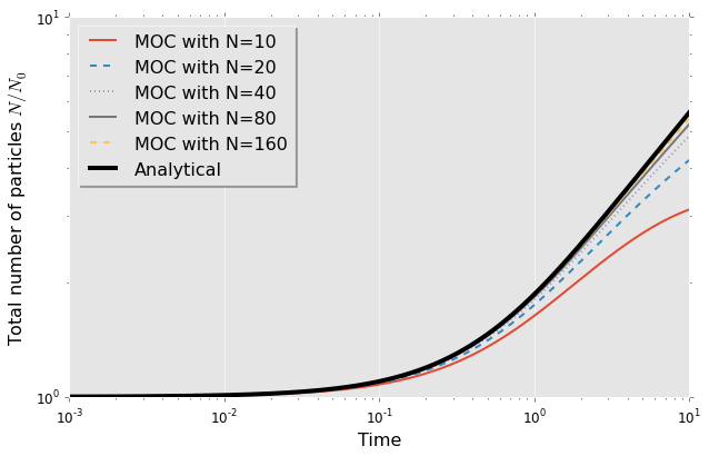
Finally we plot the results on log, log axes. The total numbers are normalised with respect to initial total number.
1 2 3 4 | |

A clear convergence to the analytical solution is visible. The figure reveals that the numerical solutions contain fewer drops then the analytical solutions. This is due to the fact that the smallest class continues to break up but there are no smaller classes represented in the discrete form so the drops are vanishing. In the end all numerical solutions will depart from the analytical curve due to that lower limit. This behaviour is already visible for $N=10$ case.
1 2 3 4 | |

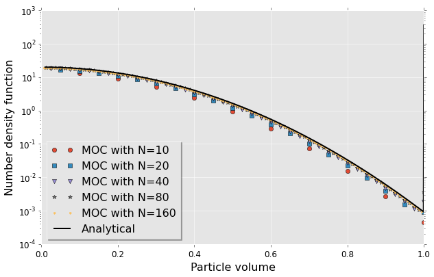
Again we observe that there’s a clear convergence to analytical solution. The visualisation of the right end of the analytical solution is somewhat problematic as it’s supposed to have a Dirac’s delta value. Don’t know how to solve presently.
Class convergence for pure agglomeration
Analytical solutions
Scott (1968) provided a solution for a pure agglomeration case with three different coalescence kernels: sum, product and constant. I will only do a constant here although I intend to add the remaining two into my test suite. In our formulation Scott’s case is
and the remaining kernels are zero.
Also, Scott assumed two types of initial conditions a dual-dispersed case with a sum of two Dirac’s deltas and a Gaussian-like distribution. In this study we will only use the latter. We use a special form of it which corresponds to setting $\nu=1$ and $a=1$ from Scott’s formulation:
It is important to observe here - and this observation cost me three hours of my life - that the mean volume from that distribution is tied to $v_2$ by $v_0 = 2v_2$. The analytical solution given by Scott for the total number is then:
where $T$ is the non-dimensional time. For the number density function the solution is:
where $\xi = v / v_0$. Below my python implementation of this for a fixed number of expansion terms.
1 2 3 4 5 6 7 8 9 10 11 12 13 14 15 | |
Numerical solutions
Similarly to previous section we set five different grids and a simulation
time. We set the simulation time to be smaller as the particles will keep
increasing its size and therefore can leave our uniform grid if enough time has
passed. vmax is set only for visualisation purpose.
1 2 3 4 5 6 7 8 9 10 11 12 13 14 15 16 17 18 19 20 21 22 | |

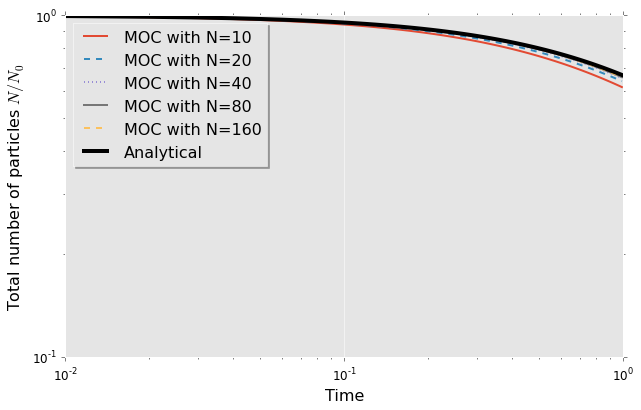
1 2 3 4 5 | |

Summary
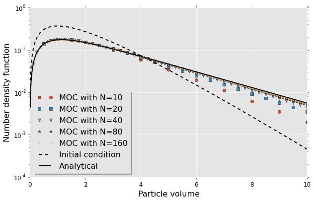
So far we can see that we have convergence to the analytical solutions. The number of classes though had to be large in comparison with what we can feasibly support in a CFD code. If method of classes is to be applied in two-fluid model it would mean solving an additional $N$ transport equations where $N$ is the number of classes and this has to be multiplied by a number of cells which probably limit our applicability to around 40 classes. The would represent a very accurate but also computationally expensive solution to the problem of population balance. This is why there is interest in developing special discretisation strategies or various methods of moments. Book by Marchiso and Fox reviews many of these other approaches. Method of classes though could be used as a validation test.
This page is still work in progress. I intend to include:
- more explanations and context,
- discussion on the challenges of PBE,
- simultaneous breakup and coalescence based on Blatz and Tobolsky,
- moment evolution.
The page acts as demonstration of the code that is being developed in pyfd repository.
References
- Smoluchowski, M. V. (1916). Drei Vortrage uber Diffusion, Brownsche Bewegung und Koagulation von Kolloidteilchen. Zeitschrift Fur Physik, 17, 557–585.
- Hidy, G. M., & Brock, J. R. (1965). Some remarks about the coagulation of aerosol particles by Brownian motion . Journal Of Colloid Science , 20(6), 477–491. doi:http://dx.doi.org/10.1016/0095-8522(65)90030-9
- Scott, W. (1968). Analytic Studies of Cloud Droplet Coalescence I. Journal Of Atmospheric Studies, 25, 54–65.
- Ziff, R. M., & McGrady, E. D. (1985). The kinetics of cluster fragmentation and depolymerisation. Journal Of Physics A: Mathematical and General, 18(15), 3027. Retrieved from http://stacks.iop.org/0305-4470/18/i=15/a=026
- Kumar, S., & Ramkrishna, D. (1996). On the solution of population balance equations by discretization—I. A fixed pivot technique. Chemical Engineering Science, 51(8), 1311–1332.
- Solsvik, J., & Jakobsen, H. A. (2015). The Foundation of the Population Balance Equation: A Review. Journal Of Dispersion Science and Technology, 36(4), 510–520. doi:10.1080/01932691.2014.909318